#Basics of Neural Networks and Deep Learning - Part 3
Course Overview: Deep Learning Course - Overview
In this course, we will learn how Neural Networks look like, and how we transform our data, so a NN can process it.
#Content of this block
The marked article is the current one.
- Our Brain and the Perceptron
- MNIST, and why good data is so important
- Structure of a Neural Network
- A Neural Network is learning
- Backpropagation
#Basic Structure of a Neural Network
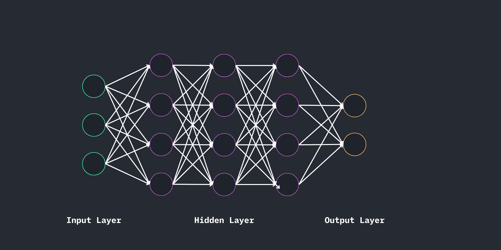
Ok, so this is how an deep neural network looks like. We have an input layer, where all our information is feeded to the NN, then a hidden layer. In the image we have only a few layers, but in reality there are usually more than three, depending on the complexity of the problem. (for our first NN we are gonna only need a few layers, but big LLM for example need much much more)
At the end there is the output layer, where we get the probabilities for the possible solutions. This will look something like that:
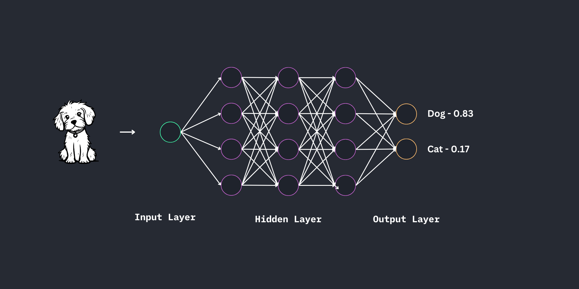
#Output Layer
(I'm just starting with the detailed expl. of the output because it's easier to explain.)
We have two output neurons, which can return a number between 0 and 1. (Note that the in and outputs are not binary anymore) Every neuron is standing for one possible solution.
You can change this, e.g. only one output neuron, and in another example with more outputs maybe something like 0 for dog, 1 for cat, 2 for turtle, 3 for octopus, and so on.
In our example in the picture we could also use only one output neuron, but as we will use one for every solution in our first project I did it here too.
Further reading, but we'll talk about this later too.
#Input Layer
How we get data into our NN depends on the application. If you're planning on coding a LLM, you'll definitly need an other input layer than for computer vision. Regarding our first project, we will look at computer vision here.
We will have one neuron for every pixel of the image we want to feed to the NN, i.e. 28 x 28 = 784 (the image has 28x28 px) input neurons. As the MNIST images of our first project are B&W, we have only one value between 0 and 255 for every pixel.
Before giving all our data to the NN, we will normalize it. This means we will take every input, and give it a value between 0 and 1.
This is not too important right now, but if we have different types of input, it will become important.
An explanation I copied from StackOverflow:
" In a nutshell, normalization reduces the complexity of the problem your network is trying to solve. This can potentially increase the accuracy of your model and speed up the training. You bring the data on the same scale and reduce variance. None of the weights in the network are wasted on doing a normalization for you, meaning that they can be used more efficiently to solve the actual task at hand. "
Example:
A NN should decide whether a elephant is male or female. Inputs are height in kilometers, and weight in milligrams, e.g. we will have sth like
height: 0.0043km; weight: 100000000mg.This makes it very hard for the NN to balance the importance of the height/weight. If we divide both values through the average value, the NN won't have to use neurons for balancing the weight of the two inputs.
In our first project it's going to be easier,
as we know a minimal (0) and maximal (255) value.
Because of this, we'll just divide all our inputs by 255.
#Hidden Layer
This is the layer where all the magic happens, and also the layer we know the least about. (The name has a reason)
Even if it's a crustBox, we know that there are many neurons, with changing thresholds and weights, that adjust parameters while training to fit the data.
One of the things we can control in the hidden layers are the types of layers we use.
We can for example connect every neuron of one layer with every neuron of the next layer,
or maybe only a few ones.
Also we can take 50 neurons in the first layer and maybe 250 in the enxt one...
This will look something like this later:
model.add(Conv2D(32, kernel_size=(3, 3), activation='relu', input_shape=(28, 28, 1)))
model.add(Conv2D(64, kernel_size=(3, 3), activation='relu'))
model.add(MaxPooling2D(pool_size=(2, 2)))
model.add(Dropout(0.25))
model.add(Flatten())
model.add(Dense(128, activation='relu'))
model.add(Dropout(0.5))
model.add(Dense(10, activation='softmax'))
We'll talk more about this in the next block when introducing keras etc.
#The End
Well, this was rather a small article, so let's jump right into the next one on NNs learning. (I'll add the link when done)
Next Article: work in progress...